RPR Frame Canonicalization for Vector KRR#
In J. Martinka, M. Pederzoli, M. Barbatti, P. O. Dral, J. Pittner, A simple approach to rotationally invariant machine learning of a vector quantity, J. Chem. Phys. 161, 174104 (2024). DOI: 10.1063/5.0230176 the authors present a simple pre and post processing heuristic to train a KRR model for prediction of challenging vector quantities. This method is called the RPR. RPR (Rotate-Predict-Rotate) transforms each geometry into a canonical inertia-tensor frame before computing descriptors and rotates the predictions back to the lab frame, ensuring equivariant predictions.
This example compares 4 variants for predicting electronic dipole moments, showing how RPR and the learnable coupling matrix from the previous example matrix each contribute. These variants are
Isotropic VectorKRR (baseline)
Coupled VectorKRR (learnable output covariance)
RPR + Isotropic VectorKRR
RPR + Coupled VectorKRR (spoiler, turns out to be the best). In this example we show these methods for a single fidelity case.
Imports#
[1]:
import numpy as np
import matplotlib.pyplot as plt

from mfml_qc.datasets import load_nitrophenol_data
from mfml_qc.representations import compute_flat_coulomb
from mfml_qc.vector_krr import VectorKRR, CoupledVectorKRR
from mfml_qc.rpr import RPRVectorKRR
Load and Split Data#
We use the highest-fidelity electronic dipole moments from QeMFi nitrophenol. Non-RPR models use pre-computed Coulomb matrices; RPR models take flattened Cartesian coordinates and compute descriptors internally after ‘canonical’-ization (it is a funny word).
[2]:
dataset = load_nitrophenol_data()
R = dataset["R"]
Z = dataset["Z"]
X_CM = dataset["X_CM"]
DPe_hf = dataset["DPe"][:, -1, :]

N_TRAIN = 512
N_TEST = 3000
KERNEL = "gaussian"
SIGMA = 250.0
REG = 1e-10

rng = np.random.RandomState(42)
perm = rng.permutation(len(DPe_hf))
train_idx, test_idx = perm[:N_TRAIN], perm[N_TRAIN : N_TRAIN + N_TEST]

X_train_cm = X_CM[train_idx]
X_test_cm = X_CM[test_idx]
X_train_flat = R[train_idx].reshape(N_TRAIN, -1)
X_test_flat = R[test_idx].reshape(N_TEST, -1)
Y_train = DPe_hf[train_idx]
Y_test = DPe_hf[test_idx]
Y_mean = np.mean(Y_train, axis=0)
Y_train_c = Y_train - Y_mean
Train All 4 Models#
We train four variants to isolate the effect of RPR and the learnable output covariance matrix. Non-RPR models operate on Coulomb matrices directly, while RPR models carry out canonicalization each geometry first.
[3]:
models = {}

m = VectorKRR(kernel_type=KERNEL, sigma=SIGMA, reg=REG)
m.train(X_train_cm, Y_train_c)
models["Isotropic"] = m.predict(X_test_cm) + Y_mean

m = CoupledVectorKRR(
    kernel_type=KERNEL, sigma=SIGMA, reg=REG, val_fraction=0.15, max_opt_iter=500
)
m.train(X_train_cm, Y_train_c)
models["Coupled T"] = m.predict(X_test_cm) + Y_mean

inner = VectorKRR(kernel_type=KERNEL, sigma=SIGMA, reg=REG)
m = RPRVectorKRR(inner, Z, compute_flat_coulomb)
m.train(X_train_flat, Y_train_c)
models["RPR+Iso"] = m.predict(X_test_flat) + Y_mean

inner = CoupledVectorKRR(
    kernel_type=KERNEL, sigma=SIGMA, reg=REG, val_fraction=0.15, max_opt_iter=500
)
m_rpr_t = RPRVectorKRR(inner, Z, compute_flat_coulomb)
m_rpr_t.train(X_train_flat, Y_train_c)
models["RPR+Coupled T"] = m_rpr_t.predict(X_test_flat) + Y_mean
Evaluate#
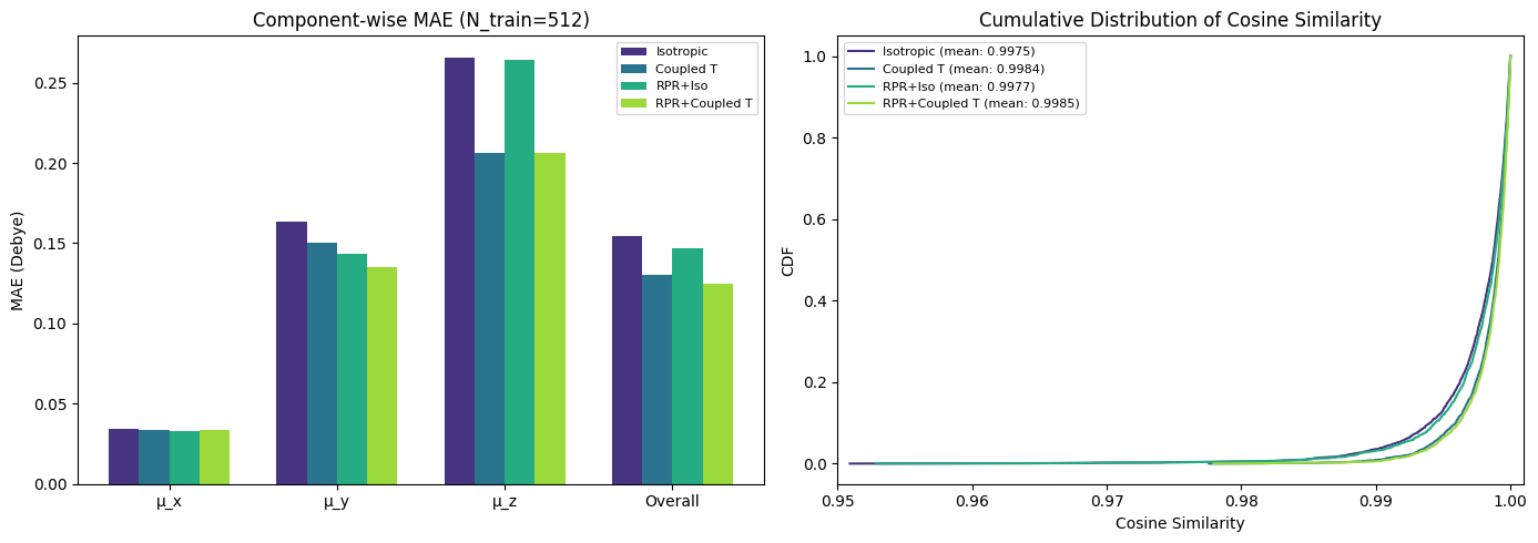
For each model we compute component-wise MAE, overall MAE, cosine similarity, and mean angular error between predicted and reference dipole vectors.
[4]:
def eval_model(name, pred, true):
    comp_mae = np.mean(np.abs(pred - true), axis=0)
    overall = np.mean(np.abs(pred - true))
    mag_p, mag_t = np.linalg.norm(pred, axis=-1), np.linalg.norm(true, axis=-1)
    dot = np.sum(pred * true, axis=-1)
    cos_sim = np.clip(dot / np.maximum(mag_p * mag_t, 1e-12), -1.0, 1.0)
    angle = np.mean(np.degrees(np.arccos(cos_sim)))
    return comp_mae, overall, cos_sim


results = {}
for name, pred in models.items():
    results[name] = eval_model(name, pred, Y_test)
Summary Plot#
The left panel shows component-wise and overall MAE for all four models. The right panel shows the cumulative distribution of cosine similarity, indicating how well each model captures dipole direction.
[5]:
names = list(models.keys())
colors = plt.cm.viridis(np.linspace(0.15, 0.85, 4))
comp_labels = ["μ_x", "μ_y", "μ_z", "Overall"]

fig, (ax1, ax2) = plt.subplots(1, 2, figsize=(14, 5))

x = np.arange(len(comp_labels))
w = 0.18
for j, name in enumerate(names):
    vals = list(results[name][0]) + [results[name][1]]
    ax1.bar(x + (j - 1.5) * w, vals, w, label=name, color=colors[j])
ax1.set_xticks(x)
ax1.set_xticklabels(comp_labels)
ax1.set_ylabel("MAE (Debye)")
ax1.set_title(f"Component-wise MAE (N_train={N_TRAIN})")
ax1.legend(fontsize=8)

for j, name in enumerate(names):
    sorted_cos = np.sort(results[name][2])
    cdf = np.arange(1, len(sorted_cos) + 1) / len(sorted_cos)
    ax2.plot(
        sorted_cos,
        cdf,
        label=f"{name} (mean: {np.mean(results[name][2]):.4f})",
        color=colors[j],
        lw=1.5,
    )
ax2.set_xlabel("Cosine Similarity")
ax2.set_ylabel("CDF")
ax2.set_title("Cumulative Distribution of Cosine Similarity")
ax2.legend(fontsize=8, loc="upper left")
ax2.set_xlim([0.95, 1.001])

plt.tight_layout()
plt.show()