A Multi-Fidelity Dataset: MD Benzene

This tutorial covers the basics of data handling, visualization, and structural representation generation in MFML-QC. We will use an inbuilt dataset for the benzene molecule.

Dataset Details

The dataset for benzene is taken from the work presented in J. Chem. Theory Comput. 2023, 19, 21, 7658–7670 (10.1021/acs.jctc.3c00882). The dataset consists of 15,000 fs MD-simulation of benzene with details of simulation presented in the article above. For the geometries of this simulation, a sparse multifidelity dataset of excitation energies is provided. Below (and in a few more tutorials) we will interact with this toy dataset to better understand the MFML-4-QC package.

Downloading the Dataset

The Benzene dataset is built into the package to allow for quick benchmarking. If you encounter a FileNotFoundError during this tutorial, ensure you have installed the package using pip install . from the root directory so the dataset is correctly packaged, or manually place the data files inside the data/benzene directory.

Loading the Built-in Dataset

We start by loading the built-in dataset using our provided utility function. This automatically handles path resolution and caching for you. Note that a cached unsorted Coulomb Matrix for all 15,000 geometries will be generated.

import numpy as np
import matplotlib.pyplot as plt
from mfml_qc.datasets import load_benzene_data

dataset = load_benzene_data()

# Let's inspect what the dataset dictionary contains.
print(f"Keys in dataset: {list(dataset.keys())}")
print(f"Columns in CSV: {dataset['columns']}")

Keys in dataset: ['X_CM', 'energies', 'timecosts', 'columns']
Columns in CSV: ['Time', 'ZINDO', 'LC-DFTB', 'STO-3G', '3-21G', '6-31G', 'def2-SVP', 'def2-TZVP', 'def2-QZVP']

Exploring the Data

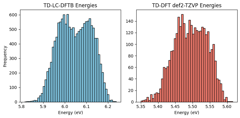
The data consists of vertical excitation energies computed at multiple fidelities and their corresponding computational time costs. Let’s extract them and look at the distributions.

energies = dataset["energies"]
timecosts = dataset["timecosts"]

# From our columns list, LC-DFTB is at index 2, and def2-TZVP is at index 7.
lc_dftb_energies = energies[:, 2]
def2_tzvp_energies = energies[:, 7]

# Drop NaN values for the plot
# (high-fidelity calculations are sparsely computed)
lc_dftb_clean = lc_dftb_energies[~np.isnan(lc_dftb_energies)]
def2_tzvp_clean = def2_tzvp_energies[~np.isnan(def2_tzvp_energies)]

fig, (ax1, ax2) = plt.subplots(1, 2, figsize=(8, 4))

ax1.hist(lc_dftb_clean, bins=50, color="skyblue", edgecolor="black")
ax1.set_title("TD-LC-DFTB Energies")
ax1.set_xlabel("Energy (eV)")
ax1.set_ylabel("Frequency")

ax2.hist(def2_tzvp_clean, bins=50, color="salmon", edgecolor="black")
ax2.set_title("TD-DFT def2-TZVP Energies")
ax2.set_xlabel("Energy (eV)")

plt.tight_layout()
plt.show()

Why Multi-Fidelity Machine Learning?

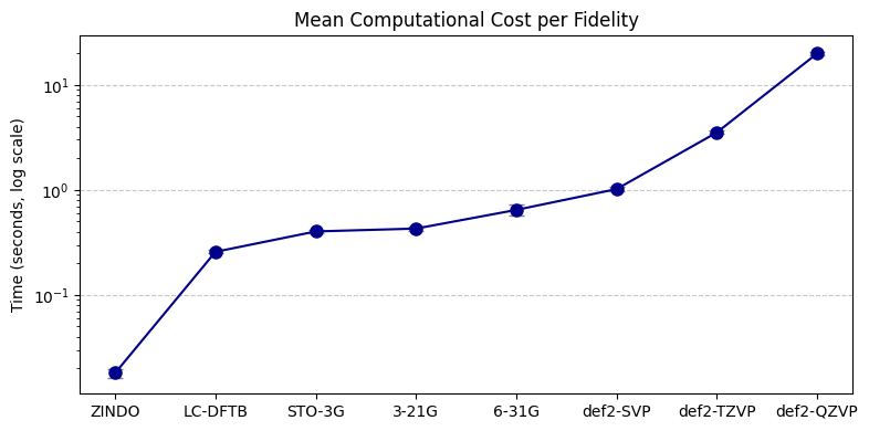
Multi-fidelity machine learning relies on the fact that lower levels of theory are significantly cheaper to compute. Let’s visualize the computational time cost distributions across all fidelities to see if we can make a case for MFML.

To ensure a fair comparison, we will extract a strict subset of geometries from the training set (the first 12,288 samples) where the most expensive calculation (def2-QZVP) is present.

train_energies = energies[:12288]
train_timecosts = timecosts[:12288]

# def2-QZVP is at column index 8.
# We create a mask for rows where it is present.
valid_qzvp_mask = ~np.isnan(train_energies[:, 8])
filtered_timecosts = train_timecosts[valid_qzvp_mask]

print(
    f"Found {np.sum(valid_qzvp_mask)} training geometries with complete hierarchy data."
)

methods = [
    "ZINDO",
    "LC-DFTB",
    "STO-3G",
    "3-21G",
    "6-31G",
    "def2-SVP",
    "def2-TZVP",
    "def2-QZVP",
]
method_indices = [1, 2, 3, 4, 5, 6, 7, 8]

# Calculate means and standard deviations
means = [np.mean(filtered_timecosts[:, i]) for i in method_indices]
stds = [np.std(filtered_timecosts[:, i]) for i in method_indices]

# ---------------------------------------------------------
# Plotting Mean and Std Dev
# ---------------------------------------------------------
plt.figure(figsize=(8, 4))

# Plotting with error bars
plt.errorbar(
    range(len(methods)),
    means,
    yerr=stds,
    fmt="o-",
    capsize=5,
    elinewidth=2,
    markersize=8,
    color="darkblue",
    ecolor="gray",
)

plt.xticks(ticks=range(len(methods)), labels=methods)
plt.yscale("log")
plt.title("Mean Computational Cost per Fidelity")
plt.ylabel("Time (seconds, log scale)")
plt.grid(axis="y", linestyle="--", alpha=0.7)
plt.tight_layout()
plt.show()

Found 384 training geometries with complete hierarchy data.

Generating Molecular Representations

Machine learning models generally cannot learn from raw 3D Cartesian (XYZ) coordinates directly, as they are not translationally or rotationally invariant. Instead, we map the 3D structures into a molecular descriptor called the Coulomb Matrix (CM). This is one of the simplest molecular descriptors and we will use this throughout the tutorials.

The load_benzene_data() function automatically invoked routines to compute and load these representations for us.

X_CM = dataset["X_CM"]
print(f"Total Geometries: {X_CM.shape[0]}")
print(f"Coulomb Matrix Features per geometry: {X_CM.shape[1]}")

Total Geometries: 15000
Coulomb Matrix Features per geometry: 78

Custom Datasets

If you are working with your own custom molecular dynamics trajectory (e.g., an .xyz file) instead of the built-in dataset, you can generate these representations manually.

The representations module handles the file parsing and memory allocation automatically:

from mfml_qc.representations import generate_coulomb_matrices

# This is the exact command you would use on your own data:
# X_custom_CM = generate_coulomb_matrices(
#     xyz_filepath="path/to/your/custom_trajectory.xyz",
#     save_path="optional/path/to/cache_coulomb_matrices.npy"
# )