The Basics of MFML

This example demonstrates how to use the MFML-QC package to load the built-in Benzene trajectory dataset, manually extract a multi-fidelity subset using a top-down approach (that is start with the highest fidelity then move down the fidelity hierarchy), and train an MFML model to predict high-fidelity excitation energies.

Imports and Helper Functions

Before we begin the actual MFML workflow, let’s define two helper functions. These are present in the utils script of the MFML package.

The first function parses our raw CSV arrays, mean-centers the target properties,and establishes the foundational indexes mapping arrays that link high-fidelity calculations back to their low-fidelity entries and corresponding geometries.

The second helper function handles Top-Down Nested Extraction. Because the provided benzene datasets is sparsely populated at high fidelities, a top-down extraction of the data guarantees that any geometry selected for a high-fidelity training set is strictly included in all lower-fidelity training sets beneath it. Note that in practice, however, one would start from the lowest fidelity and try to build their way up from there (Such as Adaptive-MFML). This will form a separate tutorial.

import os
import numpy as np
from mfml_qc.datasets import load_benzene_data
from mfml_qc.mfml import ModelMFML
from mfml_qc.utils import build_hierarchy_arrays, top_down_subsetting

Loading and Splitting the Dataset

Let’s load the built-in Benzene dataset and split it chronologically into a training pool (the first 12,288 geometries) and a test set. We will use a 4-fidelity example which in increasing order of accuracy are LC-DFTB, TD-DFT (STO-3G), TD-DFT (def2-SVP), and TD-DFT (def2-TZVP).

dataset = load_benzene_data()

X_CM = dataset["X_CM"]
data = dataset["energies"]

# LC-DFTB (Col 2) -> STO-3G (Col 3) -> def2-SVP (Col 6) -> def2-TZVP (Col 7)
hierarchy_cols = [2, 3, 6, 7]
num_fids = len(hierarchy_cols)

train_mask = data[:, 0] < 12288
test_mask = data[:, 0] >= 12288

X_train_parent = X_CM[train_mask]
X_test = X_CM[test_mask]
data_train = data[train_mask]
data_test = data[test_mask]

print(data_train.shape, data_test.shape)

(12288, 9) (2712, 9)

Preparing the Multi-Fidelity Data

We use our helper functions to extract the full valid arrays, and then apply the top-down nested extraction to enforce our specific target sizes. Here we will use 1024 samples at LC-DFTB, 512 at STO-3G, 256 at def2-SVP, and 128 samples at def2-TZVP

y_trains, indexes, means = build_hierarchy_arrays(data_train, hierarchy_cols)
n_trains_target = [1024, 512, 256, 128]
subset_y_trains, subset_indexes = top_down_subsetting(
    y_trains, indexes, n_trains_target, seed=42
)

Instantiating the MFML Model

With our data strictly nested and formatted, we can instantiate the ModelMFML class. It will automatically build and train the 2N - 1 underlying sub-models required.

mfml_model = ModelMFML(kernel="matern", sigma=715.0, reg=1e-9, p_bar=False)

We pass the subset arrays here to train on our specific N_trains targets. In a different example where we carry out a bottom-to-top data nestedness, we will come across an internal shuffler built in for the MFML. It must be noted that shuffling of training data here is what is often called random sub-sampling. The order of the data itself in training kernel based models does not affect the model.

mfml_model.train(
    X_train_parent=X_train_parent, y_trains=subset_y_trains, indexes=subset_indexes
)

Predicting and Evaluating

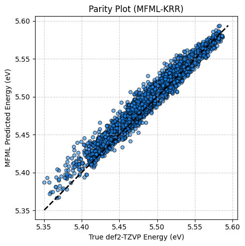
We predict the test geometries using the standard +1 and -1 weights and un-center the predictions using the highest-fidelity mean.

# Pick def2-TZVP (highest fidelity) as our "ground truth" test targets
y_test_true = data_test[:, hierarchy_cols[-1]]
preds = mfml_model.predict(X_test=X_test, optimiser="default")
preds += means[-1]

# Calculate Mean Absolute Error
mae = np.mean(np.abs(preds - y_test_true))
mae_kcal = mae * 23  # Conversion factor: eV to kcal/mol

print(f"MFML Test Set MAE: {mae:.6f} eV ({mae_kcal:.4f} kcal/mol)")

MFML Test Set MAE: 0.008261 eV (0.1900 kcal/mol)

Often, it is worth visualising a parity plot which is simply a scatter plot between the predictions and the true reference of the test set.

import matplotlib.pyplot as plt

plt.figure(figsize=(5, 5))
plt.scatter(y_test_true, preds, alpha=0.6, color="dodgerblue", edgecolor="k", s=25)

# the 45 degree diagonal indicates the ideal of everything matches perfectly
min_val = min(np.min(y_test_true), np.min(preds))
max_val = max(np.max(y_test_true), np.max(preds))
plt.plot([min_val, max_val], [min_val, max_val], "k--", lw=2)

plt.xlabel("True def2-TZVP Energy (eV)")
plt.ylabel("MFML Predicted Energy (eV)")
plt.title("Parity Plot (MFML-KRR)")
plt.grid(True, linestyle="--", alpha=0.6)
plt.tight_layout()
plt.show()