Duck Typing for MFML

This example demonstrates the “duck typing” flexibility of the ModelMFML orchestrator. DUck typing is summarized well with ‘If it walks like a duck, quacks like a duck, and swims like a duck, it must be a duck.’ Here, we use it to mean that we can use any ML architecture that has certain attributes. While MFML-QC provides an ultra-fast, built-in Kernel Ridge Regressor (KRR), you are not forced into using it.

Because the ModelMFML class is flexible, you can pass any custom machine learning model (such as a Neural Network or Random Forest from scikit-learn) using the base_estimator argument, provided it has standard .fit(X, y) or .train(X,y), and .predict(X) methods!

Imports and Helper Functions

We reuse the exact same helper functions from the previous tutorial to extract and strictly nest our multi-fidelity training data.

import os
import numpy as np
import matplotlib.pyplot as plt
from mfml_qc.datasets import load_benzene_data
from mfml_qc.mfml import ModelMFML
from mfml_qc.utils import build_hierarchy_arrays, top_down_subsetting

# We will use tha random forest regressor from scikit learn
from sklearn.ensemble import RandomForestRegressor

Loading and Splitting Data

dataset = load_benzene_data()

X_CM = dataset["X_CM"]
data = dataset["energies"]

hierarchy_cols = [2, 3, 6, 7]
num_fids = len(hierarchy_cols)

train_mask = data[:, 0] < 12288
test_mask = data[:, 0] >= 12288

X_train_parent = X_CM[train_mask]
X_test = X_CM[test_mask]
data_train = data[train_mask]
data_test = data[test_mask]

y_trains, indexes, means = build_hierarchy_arrays(data_train, hierarchy_cols)

# We use the same target sample sizes as the previous tutorial
n_trains_target = [1024, 512, 256, 128]
subset_y_trains, subset_indexes = top_down_subsetting(
    y_trains, indexes, n_trains_target, seed=42
)

Passing a Custom Base Estimator

Instead of initializing the default Kernel Ridge Regressor, we will initialize a Random Forest Regressor from scikit-learn. Before we get into the code, let’s briefly review the mechanics of a Random Forest Regressor. Unlike Kernel Ridge Regression, which relies on measuring continuous structural distances (kernels), a Random Forest is an ensemble method constructed from multiple decision trees.

For a given input geometry representation \(x\), each individual decision tree \(k\) in the forest makes an independent prediction \(h_k(x)\). The final ensemble prediction \(\hat{y}\) is simply the average of all \(K\) trees:

\begin{align}\hat{y}(x) = \frac{1}{K} \sum_{k=1}^{K} h_k(x)\end{align}

By training each tree on a random subset of the data (bootstrapping) and considering a random subset of features at each split, the Random Forest drastically reduces the variance and overfitting that is common in single decision trees.

Notice how we pass the initialized sk_model directly to the base_estimator argument of the ModelMFML object. The script will automatically duplicate this tree-based model for all 2N-1 required sub-models!

sk_model = RandomForestRegressor(
    n_estimators=50, max_depth=10, random_state=42, n_jobs=-1
)

# the mfml model class takes the random forest regressor as the base-estimator
mfml_model = ModelMFML(base_estimator=sk_model, p_bar=False)

# The class internally handles calling `.fit()` on the Random Forest models natively
mfml_model.train(
    X_train_parent=X_train_parent, y_trains=subset_y_trains, indexes=subset_indexes
)

Predicting and Evaluating

y_test_true = data_test[:, hierarchy_cols[-1]]

# the `default` optimiser carries out basic MFML
preds = mfml_model.predict(X_test=X_test, optimiser="default")

# Un-center the predictions
preds += means[-1]

mae = np.mean(np.abs(preds - y_test_true))
mae_kcal = mae * 23  # eV to kcal/mol

print(f"MFML (Random Forest) Test Set MAE: {mae:.6f} eV ({mae_kcal:.4f} kcal/mol)")

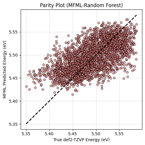
MFML (Random Forest) Test Set MAE: 0.029552 eV (0.6797 kcal/mol)

Parity Plot

We can visualize the performance of our Random Forest-based MFML model. While kernels generally perform better for molecular representations like the Coulomb Matrix, this example shows that the framework is completely model-agnostic and can be used in a modular fashion.

plt.figure(figsize=(5, 5))

# Plot the scatter points
plt.scatter(y_test_true, preds, alpha=0.6, color="lightcoral", edgecolor="k", s=25)

# Calculate the limits to draw a perfect 45-degree diagonal line
min_val = min(np.min(y_test_true), np.min(preds))
max_val = max(np.max(y_test_true), np.max(preds))
plt.plot([min_val, max_val], [min_val, max_val], "k--", lw=2)

plt.xlabel("True def2-TZVP Energy (eV)")
plt.ylabel("MFML Predicted Energy (eV)")
plt.title("Parity Plot (MFML-Random Forest)")
plt.grid(True, linestyle="--", alpha=0.6)
plt.tight_layout()
plt.show()